Linear Regression Cost function derivation

Posted by

Serge Mosin on February 22, 2018

TL;DR
From this post you’ll learn how Normal Equation derivation is performed for Linear Regression cost function.

Introduction

Recently I enrolled in wonderful Machine Learning course by Andrew Ng’s in Stanford. In the Linear Regression section, there was this Normal Equation obtained, that helps to identify cost function global minima. Unfortunately, the derivation process was out of the scope. I found it not quite obvious so I’d like to share it in case someone finds it struggling as well.

There was this post by Eli, which explains the derivation process step-by-step. However, the author performs all the Calculus in vectorized form, which is objectively more complicated that scalar one. I suggest the shorter and easier derivation process here.

Derivation

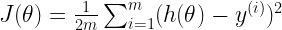
So, suppose we have cost function defined as follows:

$J(\theta) = \frac{1}{2m} \sum_{i=1}^{m}(h(\theta) - y^{(i)})^2$

The partial derivatives look like this:

$\frac{\partial J}{\partial \theta_j} = \frac{1}{m} \sum_{i=1}^{m}(\theta_0 x_0^i + \theta_1 x_1^i + \dots + \theta_n x_n^i - y^i)x_j^i,\\ j=1,\dots,n$

The set of equations we need to solve is the following:

$\frac{\partial J}{\partial \theta_j} = 0, j=1,\dots,n$

Substituting derivative terms, we get:

$\sum_{i=1}^{m}(\theta_0 x_0^i + \theta_1 x_1^i + \dots + \theta_n x_n^i - y^i)x_j^i = 0, j=1,\dots,n$

To make things more visual, let’s just decode the sigma sign and write explicitly the whole system of equations:

$\left\{ \begin{array}{c} (\theta_0 x_0^1 + \theta_1 x_1^1 + \dots + \theta_n x_n^1 - y^i)x_0^1 + (\theta_0 x_0^1 + \theta_1 x_1^1 + \dots + \theta_n x_n^1 - y^i)x_0^2 + \dots + (\theta_0 x_0^1 + \theta_1 x_1^1 + \dots + \theta_n x_n^1 - y^i)x_0^m = 0 \\ \\ \dots\\ \\ (\theta_0 x_0^1 + \theta_1 x_1^1 + \dots + \theta_n x_n^1 - y^i)x_n^1 + (\theta_0 x_0^1 + \theta_1 x_1^1 + \dots + \theta_n x_n^1 - y^i)x_n^2 + \dots + (\theta_0 x_0^1 + \theta_1 x_1^1 + \dots + \theta_n x_n^1 - y^i)x_n^m = 0 \end{array} \right.$

Let us now consider the following matrices:

$X = \begin{bmatrix} x_0^1 & x_1^1 & \dots & x_n^1 \\ x_0^2 & x_1^2 & \dots & x_n^2 \\ \dots & \dots & \dots & \dots \\ x_0^m & x_1^m & \dots & x_n^m \end{bmatrix},\ \theta = \begin{bmatrix} \theta_0 \\ \theta_1 \\ \dots \\ \theta_n \end{bmatrix},\ y = \begin{bmatrix} y_0 \\ y_1 \\ \dots \\ y_m \end{bmatrix}$

Thus, the following vector can be calculated:

$X \theta - y = \begin{bmatrix} \theta_0 x_0^1 + \theta_1 x_1^1 + \dots + \theta_n x_n^1 - y^1 \\ \dots \\ \theta_0 x_0^m + \theta_1 x_1^m + \dots + \theta_n x_n^m - y^m \end{bmatrix}$

Now, looking at our matrices and comparing them to the system of equations, we can notice that the system can be rewritten as follows:

$X^T (X \theta - y) = 0$

Simplifying, we get:

$X^T X \theta - X^T y = 0\\ X^T X \theta = X^T y\\ \theta = (X^T X)^{-1} X^T y\\$

Conclusion

Now that’s it for the day. I tried to explain algebra beneath the Linear regression Normal equation. I think it’s quite important to understand the low-level concepts of algorithms to have a better grasp of the concepts and just have a clearer picture of what’s going on. Until next time, folks. Stay cool and don’t brawl, unless with data.

References

Serge Mosin

https://www.databrawl.com/author/svmosingmail-com/

Pythonista, Data/Code lover, Apline skier and gym hitter.